Exploratory Data Analysis (EDA) Wine Quality dataset
Contents
Exploratory Data Analysis (EDA) Wine Quality dataset#
We will analyze the well-known wine dataset using our newly gained skills in this part. Each wine is described with several attributes obtained by physicochemical tests and by its quality (from 1 to 10). This dataset is perfect for many ML tasks such as:
Testing Outlier detection algorithms that can detect the few excellent or poor wines
Modeling the relationship between wine quality and wine attributes (using regression or classification)
Attribute (feature) selection techniques to remove unimportant features
✏️ The example is inspired by [Pac].
Let’s start by importing packages:
import pandas as pd
import seaborn as sns
import matplotlib.pyplot as plt
Let’s load our data (there are two datasets for red and white wines):
red_wine_url = "https://archive.ics.uci.edu/ml/machine-learning-databases/wine-quality/winequality-red.csv"
white_wine_url = "https://archive.ics.uci.edu/ml/machine-learning-databases/wine-quality/winequality-white.csv"

# load data to DF
df_red = pd.read_csv(red_wine_url, delimiter=";")
df_white = pd.read_csv(white_wine_url, delimiter=";")
Let’s check red wine data:
df_red.info()
<class 'pandas.core.frame.DataFrame'>
RangeIndex: 1599 entries, 0 to 1598
Data columns (total 12 columns):
 #   Column                Non-Null Count  Dtype
---  ------                --------------  -----
 0   fixed acidity         1599 non-null   float64
 1   volatile acidity      1599 non-null   float64
 2   citric acid           1599 non-null   float64
 3   residual sugar        1599 non-null   float64
 4   chlorides             1599 non-null   float64
 5   free sulfur dioxide   1599 non-null   float64
 6   total sulfur dioxide  1599 non-null   float64
 7   density               1599 non-null   float64
 8   pH                    1599 non-null   float64
 9   sulphates             1599 non-null   float64
 10  alcohol               1599 non-null   float64
 11  quality               1599 non-null   int64
dtypes: float64(11), int64(1)
memory usage: 150.0 KB
df_red.describe()
| fixed acidity | volatile acidity | citric acid | residual sugar | chlorides | free sulfur dioxide | total sulfur dioxide | density | pH | sulphates | alcohol | quality | |
|---|---|---|---|---|---|---|---|---|---|---|---|---|
| count | 1599.000000 | 1599.000000 | 1599.000000 | 1599.000000 | 1599.000000 | 1599.000000 | 1599.000000 | 1599.000000 | 1599.000000 | 1599.000000 | 1599.000000 | 1599.000000 |
| mean | 8.319637 | 0.527821 | 0.270976 | 2.538806 | 0.087467 | 15.874922 | 46.467792 | 0.996747 | 3.311113 | 0.658149 | 10.422983 | 5.636023 |
| std | 1.741096 | 0.179060 | 0.194801 | 1.409928 | 0.047065 | 10.460157 | 32.895324 | 0.001887 | 0.154386 | 0.169507 | 1.065668 | 0.807569 |
| min | 4.600000 | 0.120000 | 0.000000 | 0.900000 | 0.012000 | 1.000000 | 6.000000 | 0.990070 | 2.740000 | 0.330000 | 8.400000 | 3.000000 |
| 25% | 7.100000 | 0.390000 | 0.090000 | 1.900000 | 0.070000 | 7.000000 | 22.000000 | 0.995600 | 3.210000 | 0.550000 | 9.500000 | 5.000000 |
| 50% | 7.900000 | 0.520000 | 0.260000 | 2.200000 | 0.079000 | 14.000000 | 38.000000 | 0.996750 | 3.310000 | 0.620000 | 10.200000 | 6.000000 |
| 75% | 9.200000 | 0.640000 | 0.420000 | 2.600000 | 0.090000 | 21.000000 | 62.000000 | 0.997835 | 3.400000 | 0.730000 | 11.100000 | 6.000000 |
| max | 15.900000 | 1.580000 | 1.000000 | 15.500000 | 0.611000 | 72.000000 | 289.000000 | 1.003690 | 4.010000 | 2.000000 | 14.900000 | 8.000000 |
Let’s check white wine data:
df_white.info()
<class 'pandas.core.frame.DataFrame'>
RangeIndex: 4898 entries, 0 to 4897
Data columns (total 12 columns):
 #   Column                Non-Null Count  Dtype
---  ------                --------------  -----
 0   fixed acidity         4898 non-null   float64
 1   volatile acidity      4898 non-null   float64
 2   citric acid           4898 non-null   float64
 3   residual sugar        4898 non-null   float64
 4   chlorides             4898 non-null   float64
 5   free sulfur dioxide   4898 non-null   float64
 6   total sulfur dioxide  4898 non-null   float64
 7   density               4898 non-null   float64
 8   pH                    4898 non-null   float64
 9   sulphates             4898 non-null   float64
 10  alcohol               4898 non-null   float64
 11  quality               4898 non-null   int64
dtypes: float64(11), int64(1)
memory usage: 459.3 KB
df_white.describe()
| fixed acidity | volatile acidity | citric acid | residual sugar | chlorides | free sulfur dioxide | total sulfur dioxide | density | pH | sulphates | alcohol | quality | |
|---|---|---|---|---|---|---|---|---|---|---|---|---|
| count | 4898.000000 | 4898.000000 | 4898.000000 | 4898.000000 | 4898.000000 | 4898.000000 | 4898.000000 | 4898.000000 | 4898.000000 | 4898.000000 | 4898.000000 | 4898.000000 |
| mean | 6.854788 | 0.278241 | 0.334192 | 6.391415 | 0.045772 | 35.308085 | 138.360657 | 0.994027 | 3.188267 | 0.489847 | 10.514267 | 5.877909 |
| std | 0.843868 | 0.100795 | 0.121020 | 5.072058 | 0.021848 | 17.007137 | 42.498065 | 0.002991 | 0.151001 | 0.114126 | 1.230621 | 0.885639 |
| min | 3.800000 | 0.080000 | 0.000000 | 0.600000 | 0.009000 | 2.000000 | 9.000000 | 0.987110 | 2.720000 | 0.220000 | 8.000000 | 3.000000 |
| 25% | 6.300000 | 0.210000 | 0.270000 | 1.700000 | 0.036000 | 23.000000 | 108.000000 | 0.991723 | 3.090000 | 0.410000 | 9.500000 | 5.000000 |
| 50% | 6.800000 | 0.260000 | 0.320000 | 5.200000 | 0.043000 | 34.000000 | 134.000000 | 0.993740 | 3.180000 | 0.470000 | 10.400000 | 6.000000 |
| 75% | 7.300000 | 0.320000 | 0.390000 | 9.900000 | 0.050000 | 46.000000 | 167.000000 | 0.996100 | 3.280000 | 0.550000 | 11.400000 | 6.000000 |
| max | 14.200000 | 1.100000 | 1.660000 | 65.800000 | 0.346000 | 289.000000 | 440.000000 | 1.038980 | 3.820000 | 1.080000 | 14.200000 | 9.000000 |
As we will later combine our datasets into a single one, let’s add an extra column to indicate category:
df_white['wine_category'] = 'white'
df_red['wine_category'] = 'red'
A colleague in our department, a wine expert, gave us a tip that scaling the quality from 1 to 10 might probably be too granular for certain types of analysis, and it might be OK to divide wines into three quality categories - low, medium, high:
df_red['quality_label'] = df_red['quality'].apply(lambda value: ('low' if value <= 5 else 'medium') if value <= 7 else 'high')
df_red['quality_label'] = pd.Categorical(df_red['quality_label'], categories=['low', 'medium', 'high'])

df_white['quality_label'] = df_white['quality'].apply(lambda value: ('low' if value <= 5 else 'medium') if value <= 7 else 'high')
df_white['quality_label'] = pd.Categorical(df_white['quality_label'], categories=['low', 'medium', 'high'])
Red Wine Dataset Analysis#
Let’s get familiar with the red wine dataset with some visualizations that we already know:
_, axes = plt.subplots(1, 2, figsize=(20, 5))

sns.countplot(data=df_red, x='quality', ax=axes[0])
sns.countplot(data=df_red, x='quality_label', ax=axes[1]);

Well, the dataset is highly imbalanced when it comes to quality attribute.
Let’s check some relationships between attributes:
sns.pairplot(df_red.drop(columns=['quality']), hue="quality_label", height=3);
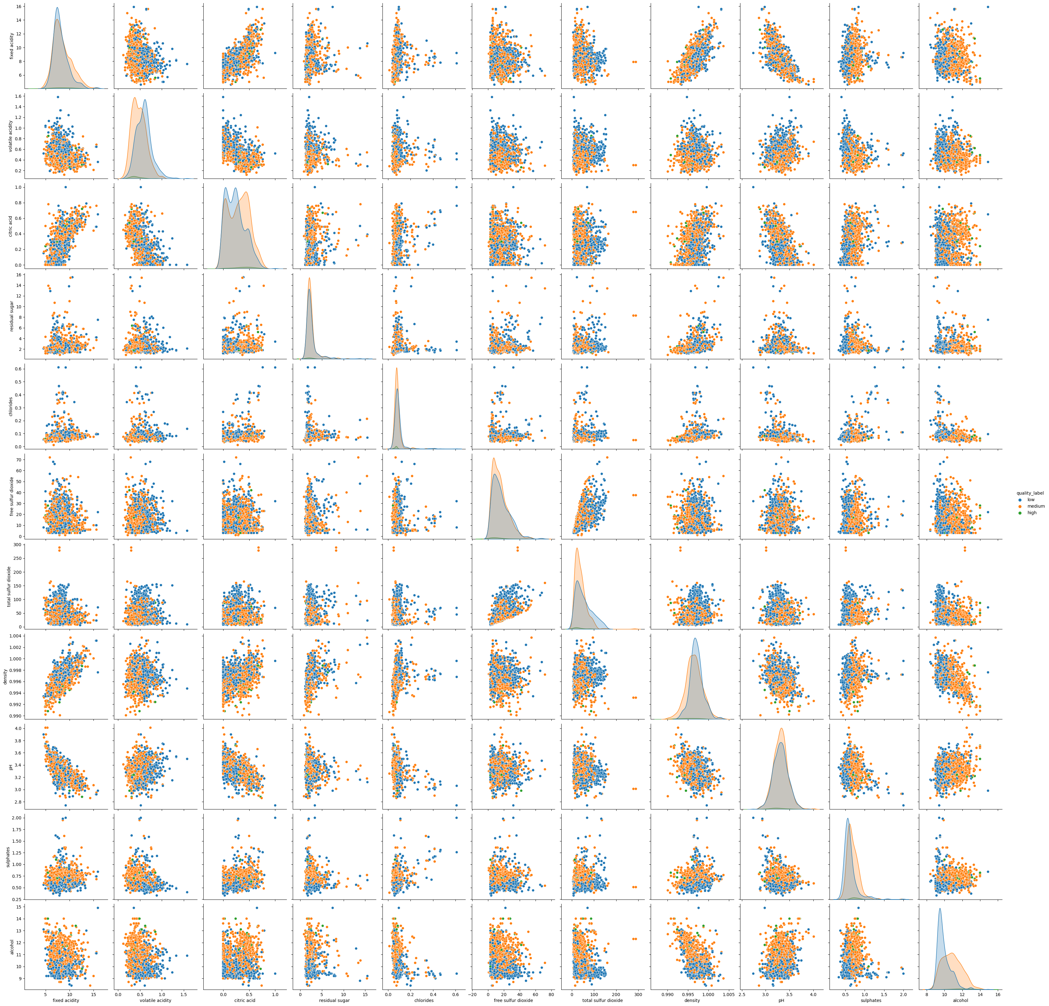
The plot is somehow hard to read. Let’s try to focus on an individual attribute:
_, axes = plt.subplots(1, 2, figsize=(10, 5))

sns.violinplot(data=df_red, y="alcohol", x="quality_label", ax=axes[0])
sns.violinplot(data=df_red, y="alcohol", x="quality", ax=axes[1]);
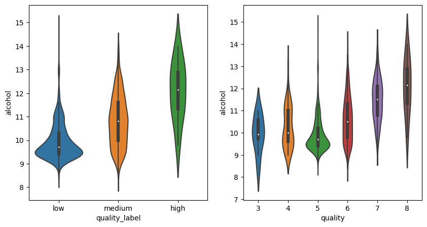
There are no obvious gotchas. Maybe we will be more lucky with the correlation plot:
sns.heatmap(df_red.corr(method="pearson"), annot=True);
/tmp/ipykernel_18914/527241991.py:1: FutureWarning: The default value of numeric_only in DataFrame.corr is deprecated. In a future version, it will default to False. Select only valid columns or specify the value of numeric_only to silence this warning.
  sns.heatmap(df_red.corr(method="pearson"), annot=True);
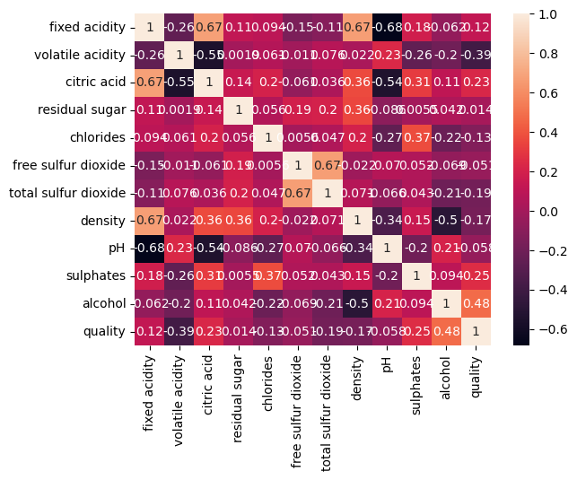
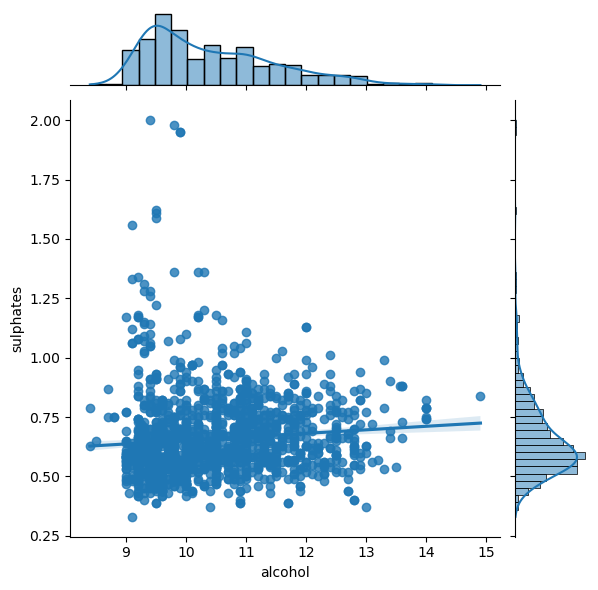
There are definitely some interactions, we can study them, for example, with jointplot:
sns.jointplot(x='alcohol',y='sulphates',data=df_red, kind='reg');
Let’s analyze relationship between attributes and the quality:
columns = list(filter(lambda col: col not in {'quality', 'wine_category', 'quality_label'}, df_red.columns))
chunks = [columns[i:i + 6] for i in range(0, len(columns), 6)]
for columns_names in chunks:
    sns.pairplot(df_red, x_vars=columns_names, y_vars='quality', kind="reg")


White Wine Dataset Analysis#
Let’s run the same analysis for the white vine:
_, axes = plt.subplots(1, 2, figsize=(20, 5))

sns.countplot(data=df_white, x='quality', ax=axes[0])
sns.countplot(data=df_white, x='quality_label', ax=axes[1]);

sns.pairplot(df_white.drop(columns=['quality']), hue="quality_label", height=3);
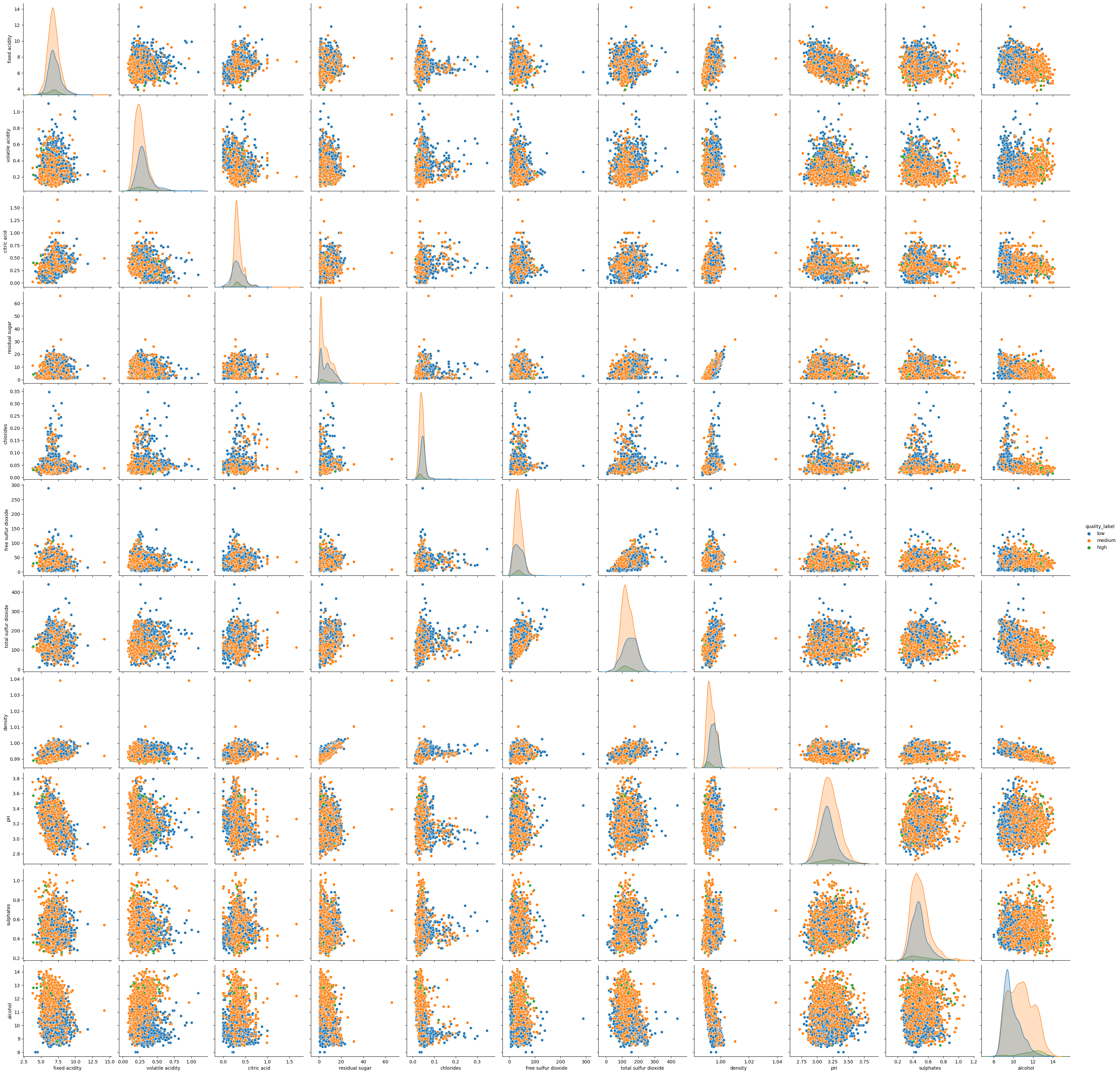
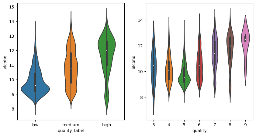
_, axes = plt.subplots(1, 2, figsize=(10, 5))

sns.violinplot(data=df_white, y="alcohol", x="quality_label", ax=axes[0])
sns.violinplot(data=df_white, y="alcohol", x="quality", ax=axes[1]);
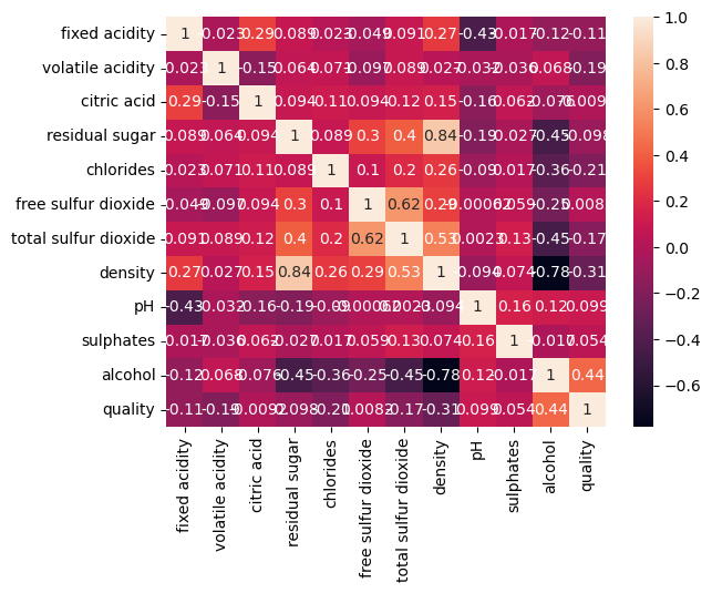
sns.heatmap(df_white.corr(method="pearson"), annot=True);
/tmp/ipykernel_18914/455693947.py:1: FutureWarning: The default value of numeric_only in DataFrame.corr is deprecated. In a future version, it will default to False. Select only valid columns or specify the value of numeric_only to silence this warning.
  sns.heatmap(df_white.corr(method="pearson"), annot=True);
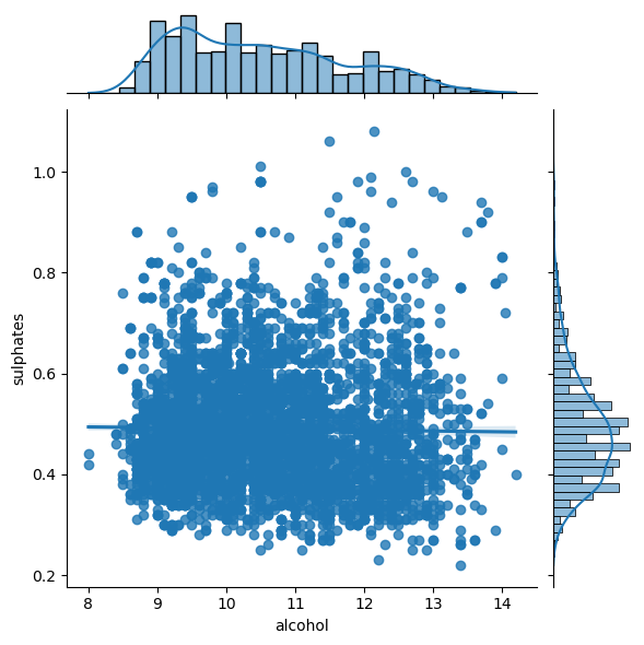
sns.jointplot(x='alcohol',y='sulphates',data=df_white, kind='reg');
columns = list(filter(lambda col: col not in {'quality', 'wine_category', 'quality_label'}, df_white.columns))
chunks = [columns[i:i + 6] for i in range(0, len(columns), 6)]
for columns_names in chunks:
    sns.pairplot(df_white, x_vars=columns_names, y_vars='quality', kind="reg")


Not surprisingly enough, white wine has a bit of different properties. Let’s combine datasets for additional analysis.
Analyze Combined Data#
Let’s concatenate datasets together:
df_wines = pd.concat([df_red, df_white])

# re-shuffle records just to randomize data points
df_wines = df_wines.sample(frac=1.0, random_state=42).reset_index(drop=True)
df_wines.head(10)
| fixed acidity | volatile acidity | citric acid | residual sugar | chlorides | free sulfur dioxide | total sulfur dioxide | density | pH | sulphates | alcohol | quality | wine_category | quality_label | |
|---|---|---|---|---|---|---|---|---|---|---|---|---|---|---|
| 0 | 7.0 | 0.17 | 0.74 | 12.8 | 0.045 | 24.0 | 126.0 | 0.99420 | 3.26 | 0.38 | 12.2 | 8 | white | high |
| 1 | 7.7 | 0.64 | 0.21 | 2.2 | 0.077 | 32.0 | 133.0 | 0.99560 | 3.27 | 0.45 | 9.9 | 5 | red | low |
| 2 | 6.8 | 0.39 | 0.34 | 7.4 | 0.020 | 38.0 | 133.0 | 0.99212 | 3.18 | 0.44 | 12.0 | 7 | white | medium |
| 3 | 6.3 | 0.28 | 0.47 | 11.2 | 0.040 | 61.0 | 183.0 | 0.99592 | 3.12 | 0.51 | 9.5 | 6 | white | medium |
| 4 | 7.4 | 0.35 | 0.20 | 13.9 | 0.054 | 63.0 | 229.0 | 0.99888 | 3.11 | 0.50 | 8.9 | 6 | white | medium |
| 5 | 7.2 | 0.53 | 0.14 | 2.1 | 0.064 | 15.0 | 29.0 | 0.99323 | 3.35 | 0.61 | 12.1 | 6 | red | medium |
| 6 | 7.5 | 0.27 | 0.31 | 17.7 | 0.051 | 33.0 | 173.0 | 0.99900 | 3.09 | 0.64 | 10.2 | 5 | white | low |
| 7 | 6.8 | 0.11 | 0.27 | 8.6 | 0.044 | 45.0 | 104.0 | 0.99454 | 3.20 | 0.37 | 9.9 | 6 | white | medium |
| 8 | 9.0 | 0.44 | 0.49 | 2.4 | 0.078 | 26.0 | 121.0 | 0.99780 | 3.23 | 0.58 | 9.2 | 5 | red | low |
| 9 | 7.1 | 0.23 | 0.30 | 2.6 | 0.034 | 62.0 | 148.0 | 0.99121 | 3.03 | 0.56 | 11.3 | 7 | white | medium |
Just by comparing the quality, you can notice a different distributions. For example, the proportion of 5 and 6 is very different for red and white:
_, axes = plt.subplots(1, 2, figsize=(20, 5))

sns.countplot(data=df_wines, x="quality", hue="wine_category", ax=axes[0])
sns.countplot(data=df_wines, x="quality_label", hue="wine_category", ax=axes[1]);

sns.pairplot(df_wines.drop(columns=['quality']), hue="wine_category", height=3);
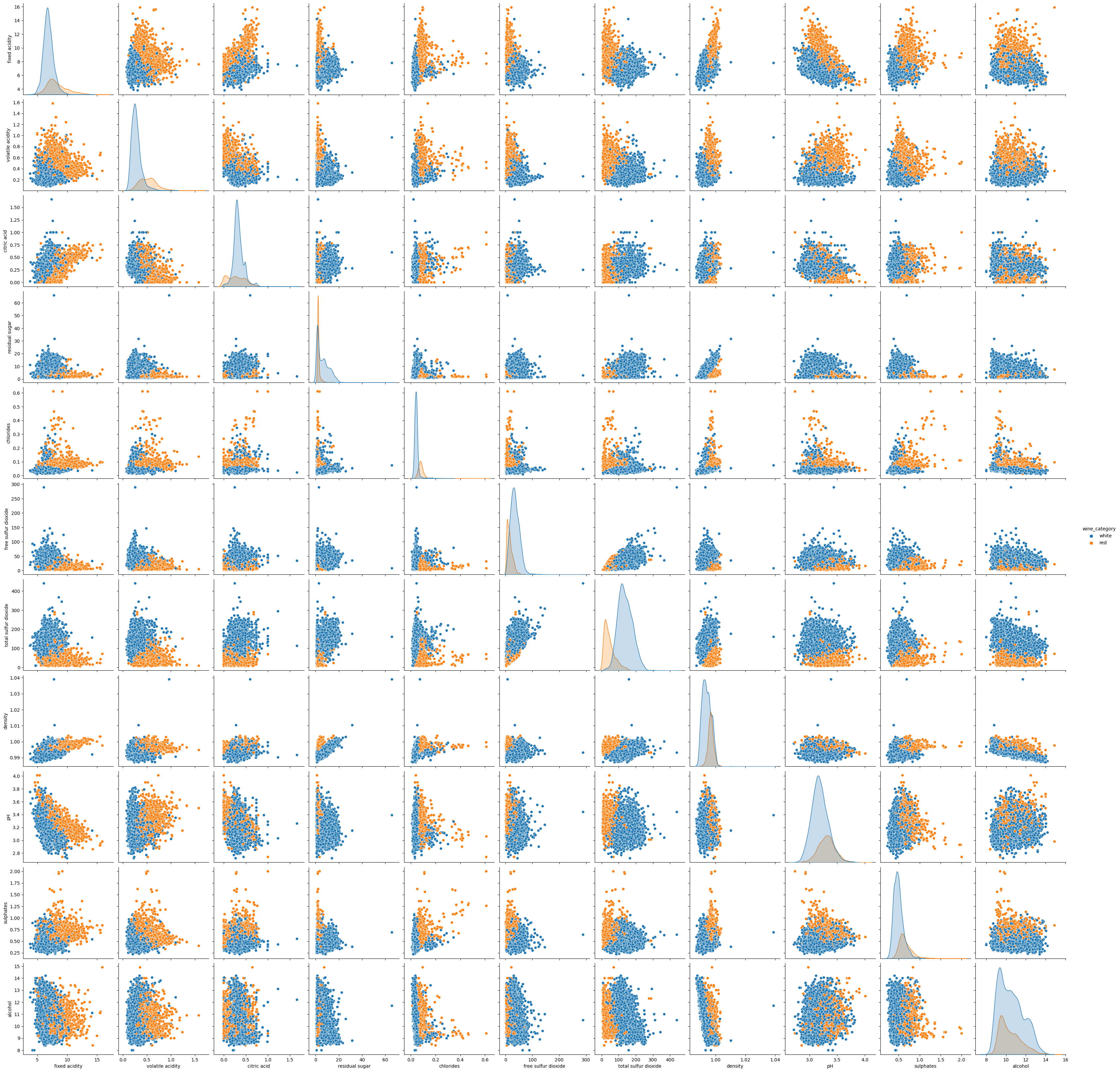
It seems that separating type of wines might be an easy task to do. Let’s check some interactions of combined dataset vs. quality:
sns.pairplot(df_wines.drop(columns=['quality']), hue="quality_label", height=3);
Error in callback <function flush_figures at 0x7f6dc92dd160> (for post_execute):
---------------------------------------------------------------------------
KeyboardInterrupt                         Traceback (most recent call last)
File ~/miniconda3/envs/ds-academy-development/lib/python3.9/site-packages/matplotlib_inline/backend_inline.py:126, in flush_figures()
    123 if InlineBackend.instance().close_figures:
    124     # ignore the tracking, just draw and close all figures
    125     try:
--> 126         return show(True)
    127     except Exception as e:
    128         # safely show traceback if in IPython, else raise
    129         ip = get_ipython()

File ~/miniconda3/envs/ds-academy-development/lib/python3.9/site-packages/matplotlib_inline/backend_inline.py:90, in show(close, block)
     88 try:
     89     for figure_manager in Gcf.get_all_fig_managers():
---> 90         display(
     91             figure_manager.canvas.figure,
     92             metadata=_fetch_figure_metadata(figure_manager.canvas.figure)
     93         )
     94 finally:
     95     show._to_draw = []

File ~/miniconda3/envs/ds-academy-development/lib/python3.9/site-packages/IPython/core/display_functions.py:298, in display(include, exclude, metadata, transient, display_id, raw, clear, *objs, **kwargs)
    296     publish_display_data(data=obj, metadata=metadata, **kwargs)
    297 else:
--> 298     format_dict, md_dict = format(obj, include=include, exclude=exclude)
    299     if not format_dict:
    300         # nothing to display (e.g. _ipython_display_ took over)
    301         continue

File ~/miniconda3/envs/ds-academy-development/lib/python3.9/site-packages/IPython/core/formatters.py:178, in DisplayFormatter.format(self, obj, include, exclude)
    176 md = None
    177 try:
--> 178     data = formatter(obj)
    179 except:
    180     # FIXME: log the exception
    181     raise

File ~/miniconda3/envs/ds-academy-development/lib/python3.9/site-packages/decorator.py:232, in decorate.<locals>.fun(*args, **kw)
    230 if not kwsyntax:
    231     args, kw = fix(args, kw, sig)
--> 232 return caller(func, *(extras + args), **kw)

File ~/miniconda3/envs/ds-academy-development/lib/python3.9/site-packages/IPython/core/formatters.py:222, in catch_format_error(method, self, *args, **kwargs)
    220 """show traceback on failed format call"""
    221 try:
--> 222     r = method(self, *args, **kwargs)
    223 except NotImplementedError:
    224     # don't warn on NotImplementedErrors
    225     return self._check_return(None, args[0])

File ~/miniconda3/envs/ds-academy-development/lib/python3.9/site-packages/IPython/core/formatters.py:339, in BaseFormatter.__call__(self, obj)
    337     pass
    338 else:
--> 339     return printer(obj)
    340 # Finally look for special method names
    341 method = get_real_method(obj, self.print_method)

File ~/miniconda3/envs/ds-academy-development/lib/python3.9/site-packages/IPython/core/pylabtools.py:151, in print_figure(fig, fmt, bbox_inches, base64, **kwargs)
    148     from matplotlib.backend_bases import FigureCanvasBase
    149     FigureCanvasBase(fig)
--> 151 fig.canvas.print_figure(bytes_io, **kw)
    152 data = bytes_io.getvalue()
    153 if fmt == 'svg':

File ~/miniconda3/envs/ds-academy-development/lib/python3.9/site-packages/matplotlib/backend_bases.py:2338, in FigureCanvasBase.print_figure(self, filename, dpi, facecolor, edgecolor, orientation, format, bbox_inches, pad_inches, bbox_extra_artists, backend, **kwargs)
   2334 try:
   2335     # _get_renderer may change the figure dpi (as vector formats
   2336     # force the figure dpi to 72), so we need to set it again here.
   2337     with cbook._setattr_cm(self.figure, dpi=dpi):
-> 2338         result = print_method(
   2339             filename,
   2340             facecolor=facecolor,
   2341             edgecolor=edgecolor,
   2342             orientation=orientation,
   2343             bbox_inches_restore=_bbox_inches_restore,
   2344             **kwargs)
   2345 finally:
   2346     if bbox_inches and restore_bbox:

File ~/miniconda3/envs/ds-academy-development/lib/python3.9/site-packages/matplotlib/backend_bases.py:2204, in FigureCanvasBase._switch_canvas_and_return_print_method.<locals>.<lambda>(*args, **kwargs)
   2200     optional_kws = {  # Passed by print_figure for other renderers.
   2201         "dpi", "facecolor", "edgecolor", "orientation",
   2202         "bbox_inches_restore"}
   2203     skip = optional_kws - {*inspect.signature(meth).parameters}
-> 2204     print_method = functools.wraps(meth)(lambda *args, **kwargs: meth(
   2205         *args, **{k: v for k, v in kwargs.items() if k not in skip}))
   2206 else:  # Let third-parties do as they see fit.
   2207     print_method = meth

File ~/miniconda3/envs/ds-academy-development/lib/python3.9/site-packages/matplotlib/_api/deprecation.py:410, in delete_parameter.<locals>.wrapper(*inner_args, **inner_kwargs)
    400     deprecation_addendum = (
    401         f"If any parameter follows {name!r}, they should be passed as "
    402         f"keyword, not positionally.")
    403     warn_deprecated(
    404         since,
    405         name=repr(name),
   (...)
    408                  else deprecation_addendum,
    409         **kwargs)
--> 410 return func(*inner_args, **inner_kwargs)

File ~/miniconda3/envs/ds-academy-development/lib/python3.9/site-packages/matplotlib/backends/backend_agg.py:520, in FigureCanvasAgg.print_png(self, filename_or_obj, metadata, pil_kwargs, *args)
    471 @_api.delete_parameter("3.5", "args")
    472 def print_png(self, filename_or_obj, *args,
    473               metadata=None, pil_kwargs=None):
    474     """
    475     Write the figure to a PNG file.
    476
   (...)
    518         *metadata*, including the default 'Software' key.
    519     """
--> 520     self._print_pil(filename_or_obj, "png", pil_kwargs, metadata)

File ~/miniconda3/envs/ds-academy-development/lib/python3.9/site-packages/matplotlib/backends/backend_agg.py:467, in FigureCanvasAgg._print_pil(self, filename_or_obj, fmt, pil_kwargs, metadata)
    462 """
    463 Draw the canvas, then save it using `.image.imsave` (to which
    464 *pil_kwargs* and *metadata* are forwarded).
    465 """
    466 FigureCanvasAgg.draw(self)
--> 467 mpl.image.imsave(
    468     filename_or_obj, self.buffer_rgba(), format=fmt, origin="upper",
    469     dpi=self.figure.dpi, metadata=metadata, pil_kwargs=pil_kwargs)

File ~/miniconda3/envs/ds-academy-development/lib/python3.9/site-packages/matplotlib/image.py:1656, in imsave(fname, arr, vmin, vmax, cmap, format, origin, dpi, metadata, pil_kwargs)
   1654 pil_kwargs.setdefault("format", format)
   1655 pil_kwargs.setdefault("dpi", (dpi, dpi))
-> 1656 image.save(fname, **pil_kwargs)

File ~/miniconda3/envs/ds-academy-development/lib/python3.9/site-packages/PIL/Image.py:2284, in Image.save(self, fp, format, **params)
   2281     filename = fp.name
   2283 # may mutate self!
-> 2284 self._ensure_mutable()
   2286 save_all = params.pop("save_all", False)
   2287 self.encoderinfo = params

File ~/miniconda3/envs/ds-academy-development/lib/python3.9/site-packages/PIL/Image.py:599, in Image._ensure_mutable(self)
    597 def _ensure_mutable(self):
    598     if self.readonly:
--> 599         self._copy()
    600     else:
    601         self.load()

File ~/miniconda3/envs/ds-academy-development/lib/python3.9/site-packages/PIL/Image.py:593, in Image._copy(self)
    591 def _copy(self):
    592     self.load()
--> 593     self.im = self.im.copy()
    594     self.pyaccess = None
    595     self.readonly = 0

KeyboardInterrupt:
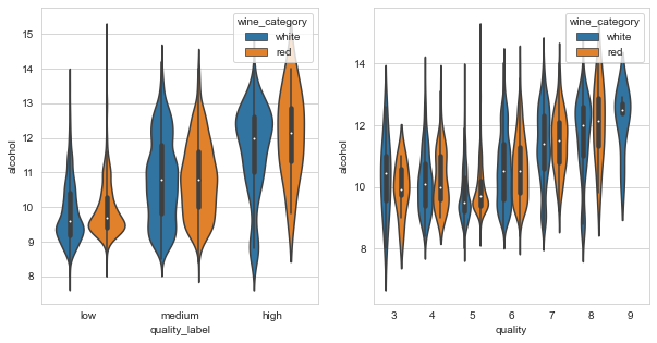
_, axes = plt.subplots(1, 2, figsize=(10, 5))

sns.violinplot(data=df_wines, y="alcohol", x="quality_label", hue="wine_category", ax=axes[0])
sns.violinplot(data=df_wines, y="alcohol", x="quality", hue="wine_category", ax=axes[1]);
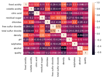
sns.heatmap(df_wines.corr(method="pearson"), annot=True);
columns = list(filter(lambda col: col not in {'quality', 'wine_category', 'quality_label'}, df_wines.columns))
chunks = [columns[i:i + 6] for i in range(0, len(columns), 6)]
for columns_names in chunks:
    sns.pairplot(df_wines, x_vars=columns_names, y_vars='quality', kind="reg")


To revisit ML tasks mentioned earlier - it is tough to tell if it is better to solve those tasks using individual datasets or the combined one based on the analysis. My bet would be to do it on individual ones, but it depends on what you want to solve and which approach you take. As always, you need to experiment. I can imagine a scenario where, for example, the smaller white wines dataset can benefit from additional data from the red wines.
✏️ Several libraries aim to automate EDA to some extent if you want to get some results as quickly as possible. One of them is pandas-profiling. An example of automated analysis is Census Dataset EDA.
Exercises#
What sorts of passengers were more likely to survive the Titanic crash?#
For the exercise, you will use the famous Titanic dataset. The sinking of the Titanic is one of the most infamous shipwrecks in history.
Unfortunately, there weren’t enough lifeboats for everyone onboard on Titanic, resulting in 1502 out of 2224 passengers and crew deaths. While some elements of luck were involved in surviving, some groups of people seemed more likely to survive than others.
# load the dataset
titanic_url = 'https://web.stanford.edu/class/archive/cs/cs109/cs109.1166/stuff/titanic.csv'
titanic_data = pd.read_csv(titanic_url)

# TODO: your answer here
Resources#
- Pac
PacktPublishing. Packtpublishing/hands-on-exploratory-data-analysis-with-python: hands-on exploratory data analysis with python, published by packt. URL: https://github.com/PacktPublishing/Hands-on-Exploratory-Data-Analysis-with-Python.

